Residue Pair Transform Scoring

Motivation for Xform Scoring

Theoretical Motivation

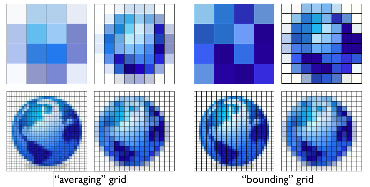
The rosetta centroid energy, by reducing each residue to a single centroid point, reduces the relationship between residues to a one dimensional distance. Many centroid-style scoring methods, including some we have and are investigating, add in an additional angle term or two (like maybe the dot product between the two CA-CB vectors), and maybe a dihedral angle, giving a 2D-4D parametrization. However, the true relationship between two protein backbone reference frames (aka stubs, analogous to centroids) is inherently a 6D geometric transform. Yet nobody uses a 6D parametrization? Why the heck not? One reason is technical difficulty, but this can be overcome. The commonly cited “scientific” reason is statistics: “there just isn’t enough data to parametrize a 6D function.” That may or may not be true for more complicated models, but what we do 90% of the time is simple binning and I would argue that for binning, it’s best to use the full dimensionality of the data. Here are two possible representations of some made-up 2D data:

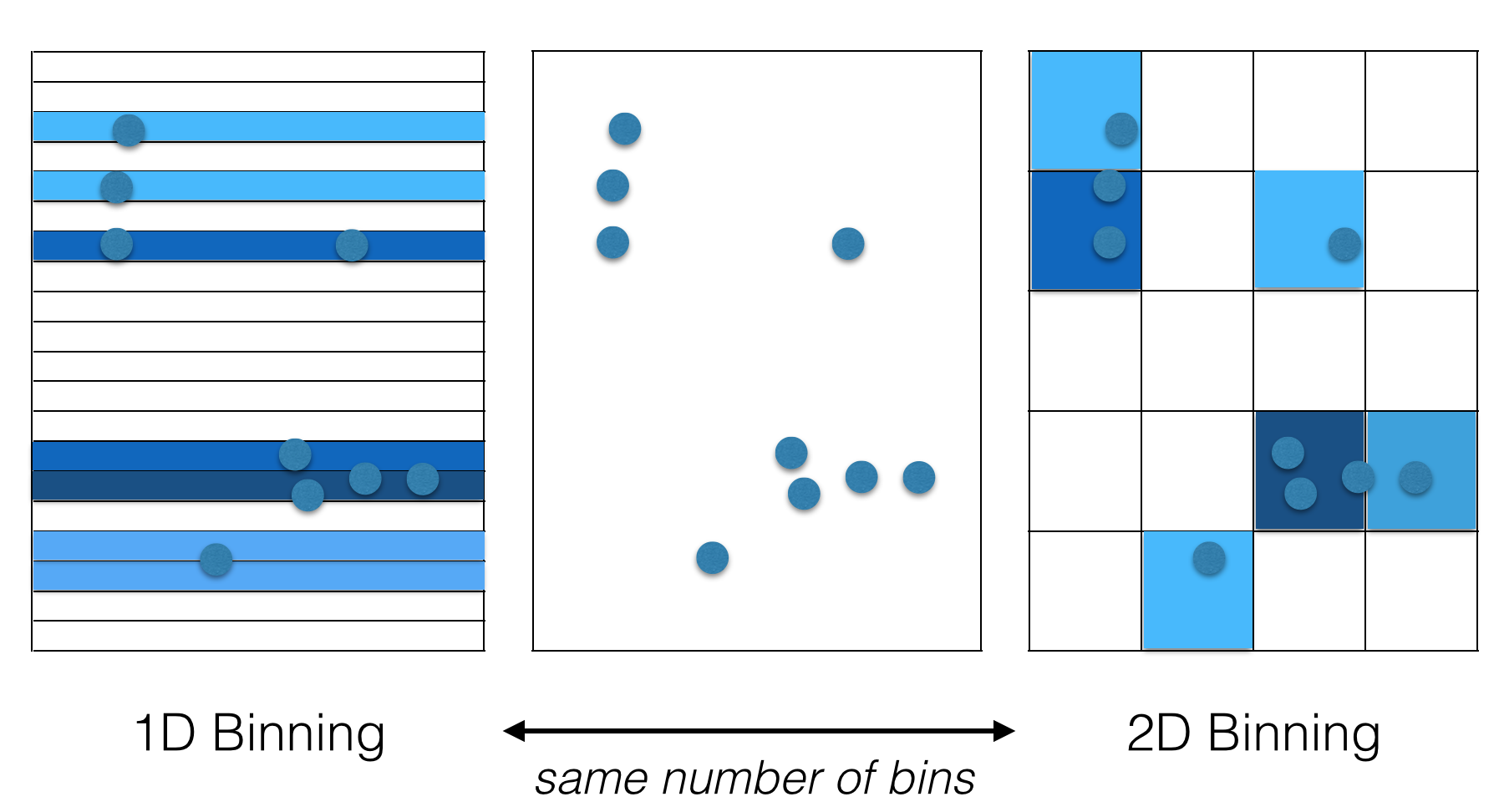
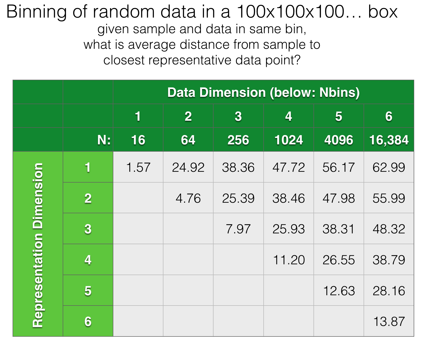
The one on the right looks much better to my eye. The key point here is that both representations use the same number of bins, so the statistical quality of the data is the same. This difference in quality becomes much more extreme as we look at higher dimensional data. Below is another totally artificial example looking at random data points in 100x100x100… boxes from 1D to 6D. In each case, we bin the data in 1..N dimensions, using the same number of bins and ask: for each binning strategy, what is the average cartesian distance from an arbitrary query point to the closest actual data point within the same bin?

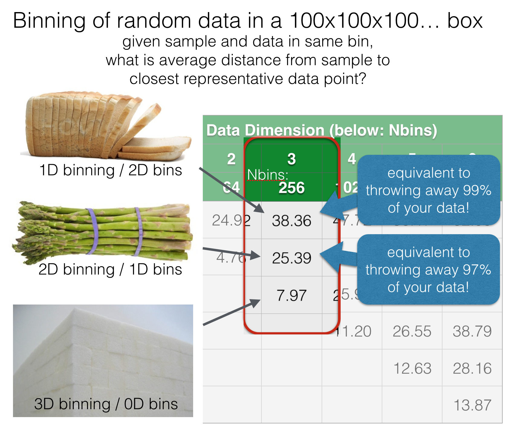
Here’s an illustration for the 3D case:

The Spherical Cow

Modeling complex objects as spheres (as we do for centroid) is the the subject of jokes:

Milk production at a dairy farm was low, so the farmer wrote to the local university, asking for help from academia. A multidisciplinary team of professors was assembled, headed by a theoretical physicist, and two weeks of intensive on-site investigation took place. The scholars then returned to the university, notebooks crammed with data, where the task of writing the report was left to the team leader. Shortly thereafter the physicist returned to the farm, saying to the farmer “I have the solution, but it only works in the case of spherical cows in a vacuum.”

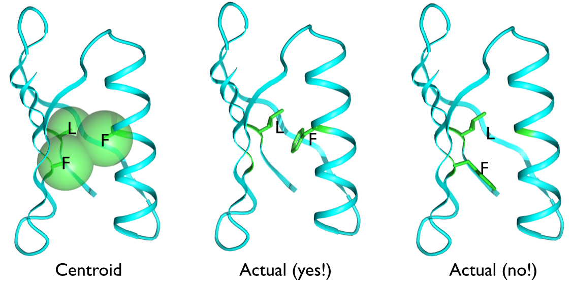
The above illustration of the core of protein G shows two LF residue pairs that look the same to the rosetta centroid energy because the centroids are almost exactly the same distance apart in both cases. But one is a highly favorable interaction with much contact area, while the other is a glancing interaction with little contact. There is no way to tell these cases apart with a 1D representation, the difference is all in the relative orientation of the two residues.

The middle panel above illustrates a representation of the residues with a full xyz coordinate frame. With such a 6D representation, these cases can be easily distinguished.

Accuracy

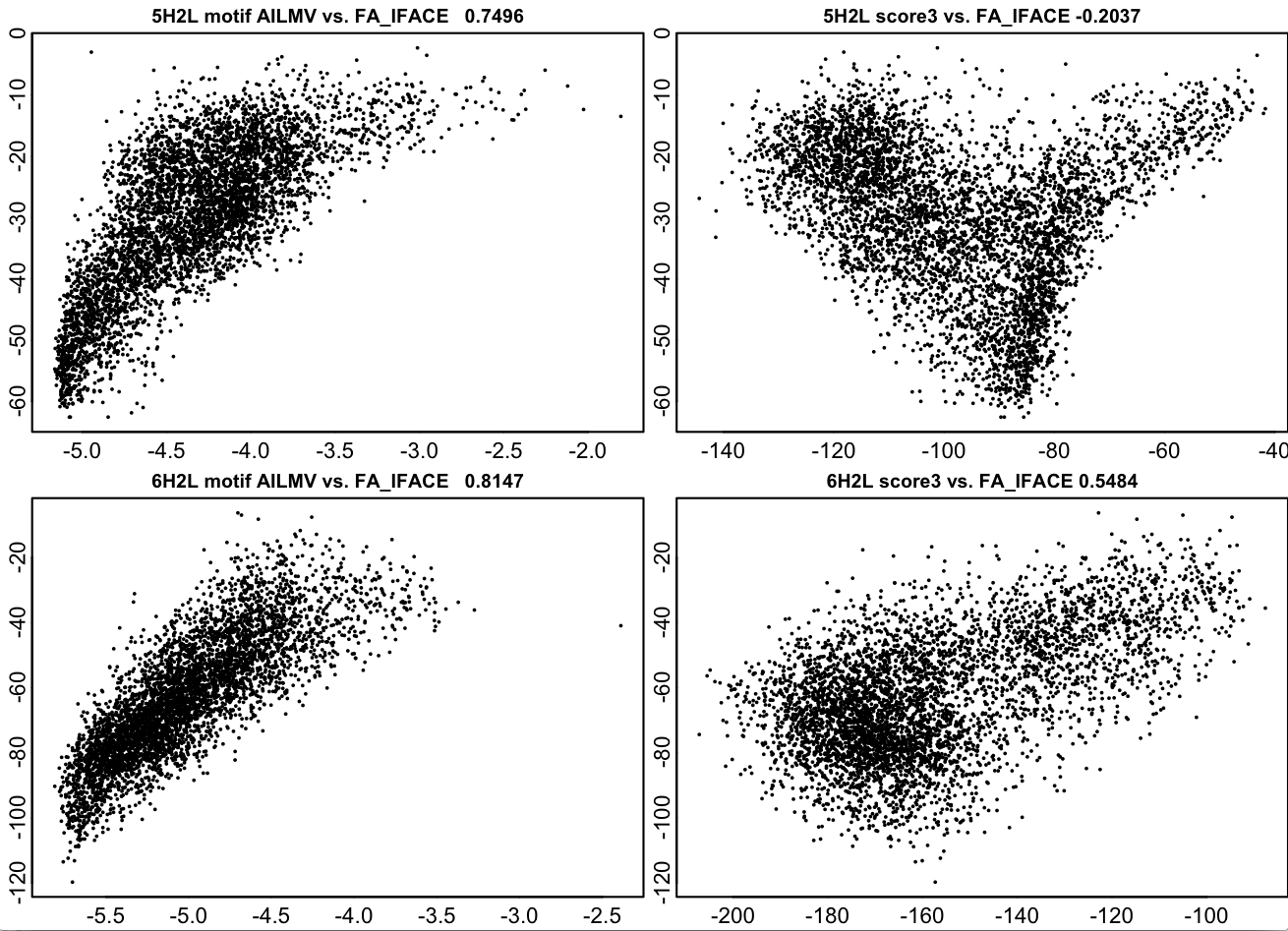
The transform based scheme score seems to be quite a bit more informative than any other “coarse grained” score I have seen. Docking prototypes based on this method seem to work very well for two sided interface design and reasonably well for some other tasks. We have not yet done much benchmarking, but hopefully will do more in the future.

The data below is for two fairly simple helical bundles of the Baker(TM) variety, one parallel one antiparallel. The plots below show Scheme and RosettaCentroid scores for backbone only structures before design plotted against Rosetta fullatom scores after a complete design process. Computing the Scheme score is approximately 10,000,000 times faster than the design calculation. These structures are close to a best-case scenario (because the interactions are helical pairs), but these are real backbones from a real project in the “wild”, not an artificial test case.

Note: people argue about what centroid residue to use to represent a pre-design structure, some use VAL, some TYR, some ALA. Here, for the sake of an argument-free comparison, I allow the centroid score to “cheat” by putting the post-design sequence on the pose. This scheme score is NOT cheating here, but the centroid score is.

Note2: design here is done without any layer design, so this is somewhat artificial.

Left panels: Scheme Score Right panels: Centroid Score X axis: Sheme / Centroid scores Y axis: Rosetta score post-design

Flexibility

This is a highly general scoring model. The “scorable” elements of a body are made up of a coordinate frames, or Actors, which may represent any arbitrary functional group. By using different Petals and different ways of building score tables, we can apply Scheme to just about any protein modeling problem that involves searching conformation space (and maybe other problem domains too).

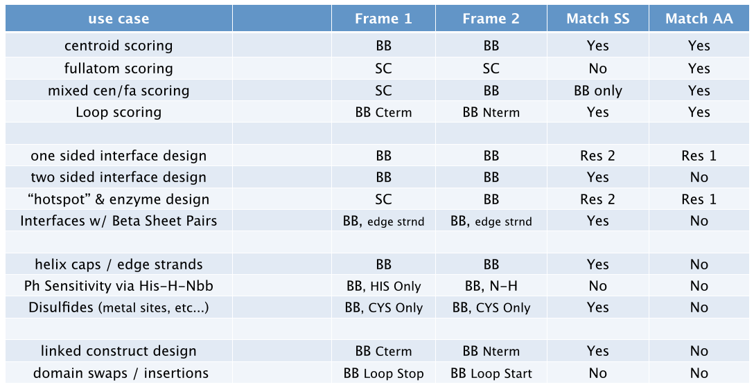
Actors

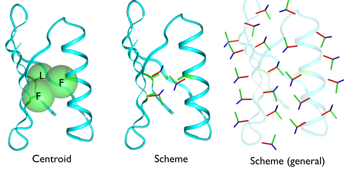
Score-able chemical entities, called Actors, are generally represented by full coordinate frames with a 3D position and orientation. The pair-score between two such entities is based on the full 6D transformation between the coordinate frames. Current Actor types are as follows. At some point, more general types will be available for hbond donors/acceptors (5dof ray), atoms (3dof xyz), and general parametric backbone systems.

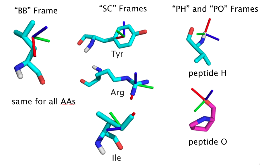
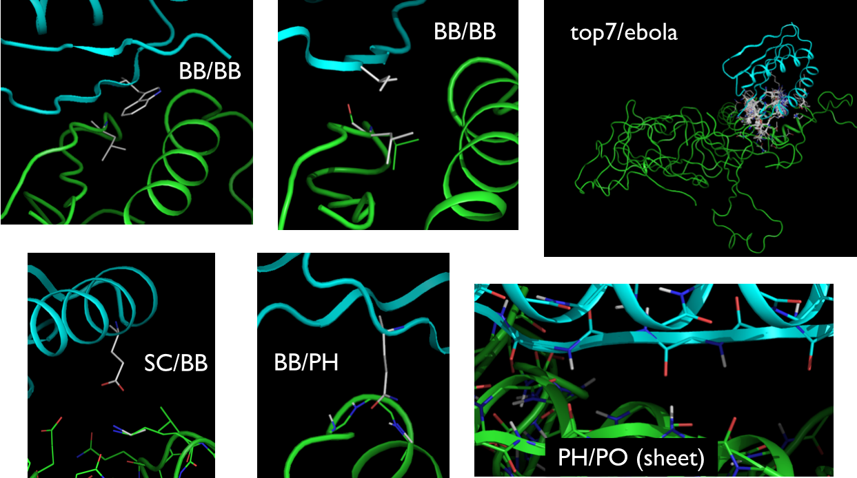
Here is an example of motifs matching various actor pair types:

Challenges

The 6D transformation space is very very large and score calculation presents some challenges The topic problem is how to score the rigid xform between a pair of “stubs” WLOG think of a pair of backbone N-Ca-C stubs and the possible side chain interactions they could allow. Native pdb motifs are pretty sparse in 6D xform space, which is a problem for polar interface design, loop design, any kind of one-sided design and even more so for structure prediction. We need more coverage to do well on these problems. Maybe we wait until the PDB is big enough, or maybe we replace or supplement with “denovo” score tables with Rosetta FA or some other continuous force field. In any case, the necessity will be much bigger score grids with trillions and trillions of data points going into them to reasonably cover the space. This is a technical challenge.

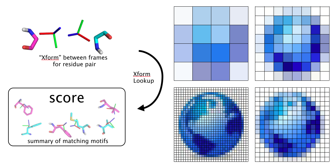
One part of the answer is hierarchal score grids; I’ll give an example using the highest resolution we might reasonably use… ~2**64 = 1.8e19 cells which gets us a resolution of 0.016A translation and 0.3° rotation (more than sufficient for sidechain interactions.. I don’t see any need for > 64bit indices in scoring). Call this G8. Obviously we can’t store, or even compute, everything in such a huge grid… It will be sparsely populated with only the very best and/or most geometrically specific (steepest gradient) interactions. If a data point (or more likely a block of 2**6 or 4**6 data points) don’t make the cut for the finest grid, it could go in the next finest grid G7, its parent, which will have ~2**58 cells at 0.032A/0.6° resolution. Each cell in the parent exactly covers 2**6 = 64 child cells, hense the 6 bit reduction in size. If not there, it could go in the next finest G6 with ~2**52 cells, or the next G5 ~2**46, and so forth to the base grid G0 with ~2**16 cells and a resolution of maybe 4.0A and about a radian. So in this instance there would be a nested hierarchy G8-G0 with 9 levels.

When looking up the score for an interaction, you must figure out the highest G which actually contains your point, then look up its score. Naively, this could require querying up to half the grids on “average”. Using some kind of skewed binary search maybe only 2 or 3. But we’d really like to make only one grid lookup because each one is expensive. This for two reasons: (1) the mapping from an RB xform to an index number is nontrivial, and (2) looking up the resulting index in memory via a hash table or whatever takes a while because there is probably a cache miss involved. The nested grid/indexing setup I’ve just finished mitigates (1) by allowing all grids G0-G8 to use basically the same index. For (2), instead of checking each one, or doing a binary search of something, a bloom filter for each resolution grid can tell you 99 times out of 100 whether the data you want is available using only maybe 65K or so of memory. (it’s an interesting data structure… worth checking out)

Hierarchical Score Grids

Scores must be computed such that they evaluate an ensemble of conformations, not just a single one. Sampling is done in a hierarchy such that each sample point must cover a defined region of space. High up in the hierarchy, a sample point would be responsible for a large volume of space, say, 5Å in diameter with orientational deviation up to 15°. Lower down in the iterative sampling hierarchy, a sample point might represent a region 0.1Å in diameter and 1° orientational deviation.

Bounding Score Grids

This, along with hierarchical decomposition, will allow implementations of Branch and Bound searches.

It is possible to construct score functions that rigorously bound the best possible score in a region of conformation space. If scoring can be set up in this manner, along with careful tracking of the volume sample points must represent, a branch and bound search is possible. Such a search would guarantee that no possible solution worse than a reported threshold was missed in the search.